When to Use What: The Missing Framework for Multi-Agent Competitive Systems

Update, October 2026: I first published this in January 2026. The framework is unchanged, but a lot has moved since. Generative auto-bidding reached production, LLM agents became competitors worth modeling, tabular foundation models changed the per-competitor step, and conformal prediction moved closer to the decision. New studies of the same Singapore data also showed that bidders drift over time and that some of them are linked by ownership. All of this is in What changed in 2026. I redrew the figures with the updates marked in teal and corrected several citations.

Summary

Competitive multi-agent problems such as auction bidding, ad placement, and trading are often approached with multi-agent reinforcement learning (MARL) or Nash equilibrium. Both assume something that rarely holds: that you can experiment online, or that your competitors are rational.

Most real settings are one-shot (a sealed bid gets no second try) and offline (you have history but cannot interact with the market). Competitors act on habits and biases, not on an equilibrium.

For these settings a simpler stack works better than MARL: behavioral cloning to model each competitor, quantile regression for the spread of their bids, conformal prediction to calibrate the intervals, and Monte Carlo simulation to choose your own bid. I validated this on Singapore’s public procurement data (900+ contractors, 8,000+ bids, 2015–2021).

The four 2×2 matrices below help decide which methods fit a given problem.

Where the framework comes from

When you build a bidding system, an ad placement optimizer, or a trading strategy, you can find papers on MARL, Monte Carlo simulation, copulas, and diffusion models. The hard part is deciding which one to use, and the usual answer is “it depends.”

I wrote this framework down after analyzing bidding systems for large government procurement auctions, where 50+ competitors bid at once on construction contracts worth $200K to $30M. The case study below uses Singapore’s public procurement data (900+ contractors, 8,000+ bids, 2015–2021).

What runs in production

Research and deployment diverge. Some examples of competitive multi-agent systems in production:

• Online advertising (Alibaba, Google Ads): RL-based bidding runs on top of models such as Deep Interest Networks. AuctionNet (NeurIPS 2024) is a benchmark for auto-bidding agents in large ad auctions. Alibaba’s sponsored-search real-time bidding system uses hour-aggregated MDPs to cope with non-stationary traffic.
• Conformal prediction for auctions: The SPACE algorithm (Lotan et al., 2024) uses conformal prediction for statistically truthful auctions, and Vijayan et al. (2025) study online bidding under return-on-spend constraints. Both treat uncertainty quantification as essential, because predictions in a noisy market are never exact.
• Energy markets: MARL-based strategic bidding adapts to real-time price changes, and agent-based simulators such as the open-source ASSUME framework use multi-agent deep RL for scenario planning in electricity markets (Harder et al., 2025).
• Ethereum MEV auctions: Flashbots MEV-Boost separates block proposers from block builders, and builders use gradient boosting and neural networks to construct blocks. BuilderNet (December 2024) decentralizes block building further. Profit is heavy-tailed: 0.1% of auctions account for 30% of total profit.

The pattern across these systems:

• simpler models such as XGBoost and LightGBM beat complex ones
• ensembles beat a single sophisticated model
• conformal calibration provides the coverage guarantees a business needs
• modeling behavior beats assuming rational opponents

Four decision matrices

Answer four questions about your problem. Each one is a 2×2 matrix that narrows the set of methods.

Matrix 1: Time structure × interaction type

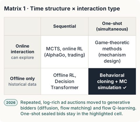
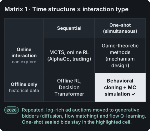
Most real competitive settings are one-shot and offline. You cannot explore; you have history and must bid well the first time. That rules out most RL methods.

Matrix 2: Agent model × output type

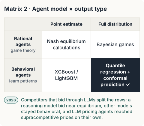
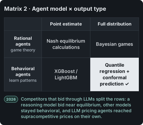
Real competitors are behavioral rather than rational. They have habits, biases, and patterns, and learning those patterns beats assuming rationality in most industrial applications.

Matrix 3: Dependence structure × scale

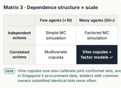
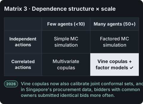
Competitors who watch the same market signals move together. Treating them as independent makes the predicted intervals too narrow.

Matrix 4: Modality × uncertainty requirements

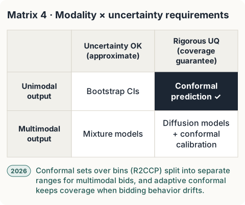
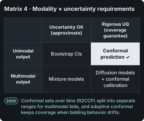
If a competitor might bid conservatively or aggressively, a single prediction hides that. You need a distribution.

The decision tree

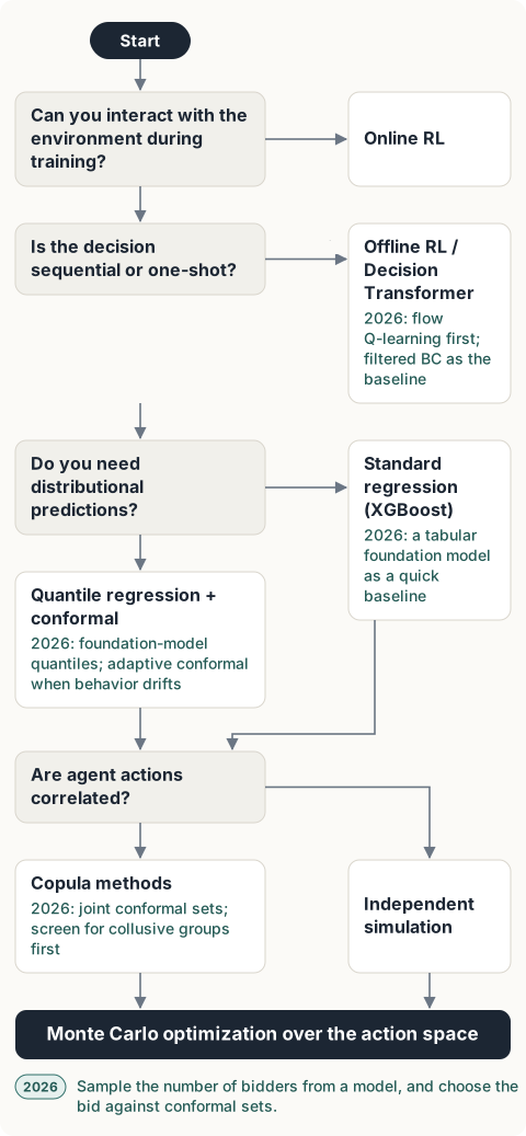
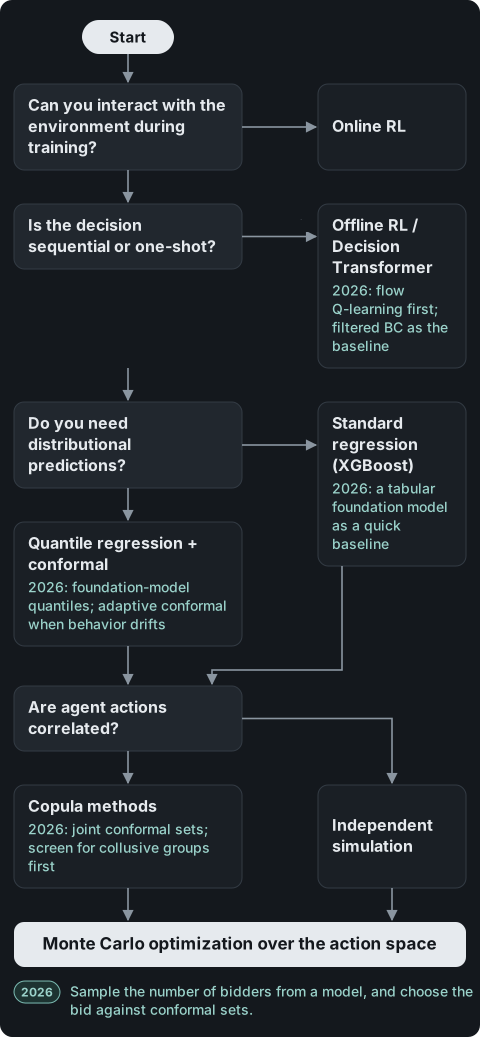
Choosing between methods

Behavioral cloning or offline RL

Kumar et al. (2022) compare the two directly. Use behavioral cloning (BC) when:

• your data looks like good demonstrations
• there is no need for trajectory stitching (combining the best parts of different rollouts)
• the mapping from action to outcome is simple
• distribution shift is small
• you need one best prediction and uncertainty does not drive the decision

Use offline RL when:

• you need trajectory stitching
• the data is suboptimal but varied
• decisions depend on each other over time
• a better policy can be extracted from mixed-quality data

For competitive bidding, BC fits. Each past bid shows what company X does in situation Y, and the goal is to forecast that behavior, not to improve it.

Trajectory stitching is where offline RL earns its place. In a maze, suppose expert A turns right at the first junction and then fails, and expert B turns left at the second junction and also fails. Offline RL can learn “right at the first, then left at the second.” BC can only imitate. Bids are independent one-shot decisions, so there is nothing to stitch, and BC plus simulation is enough.

Hybrid methods help when you start from demonstrations and want to optimize later. Cycle-of-Learning frameworks combine a BC loss with a one-step Q-learning loss and off-policy pre-training, which lets you move from BC to RL without losing performance.

Monte Carlo simulation or Monte Carlo tree search

The names are similar, but the tools solve different problems.

Monte Carlo tree search (MCTS) suits:

• sequential decisions
• a state space that can be searched as a tree
• online planning
• problems that need an exploration–exploitation balance, as in AlphaGo and game AI

Monte Carlo simulation suits:

• one-shot evaluation of known distributions
• sampling from fitted distributions and scoring the outcomes
• risk analysis and auction simulation

Sealed bids are submitted at the same time, so there is no game tree to search. When 50 companies bid at once, Monte Carlo simulation over fitted bid distributions is the right tool.

Copulas for correlated competitors

The usual approach models each competitor independently:

# Naive approach
for competitor in competitors:
    bid = model[competitor].predict(features)
    bids.append(bid)

This breaks when competitors see the same signals. A risky project makes everyone bid conservatively; a lucrative one makes everyone bid aggressively.

Use copulas when:

• competitors observe common market signals
• their past bids are strongly correlated
• tail dependence matters, because extreme events cluster
• your current model’s intervals are too narrow

Vine copulas work well for 50+ agents because they break the joint distribution into pairwise copulas, which avoids the curse of dimensionality.

Conformal prediction or bootstrap

Both give prediction intervals. Conformal prediction gives a stronger guarantee.

Bootstrap intervals:

• come from resampling
• rely on distributional assumptions that are often violated
• have approximate coverage
• are fast but can be miscalibrated

Conformal prediction:

• is distribution-free
• guarantees finite-sample coverage: a 90% interval contains the true value 90% of the time
• works with any trained model, from XGBoost to neural networks

Here is split conformal prediction on top of quantile regression:

# Split Conformal Prediction for Quantile Regression
from sklearn.model_selection import train_test_split

# 1. Split data: training + calibration
X_train, X_cal, y_train, y_cal = train_test_split(X, y, test_size=0.2)
# 2. Train quantile models (5th and 95th percentile)
model_lower = XGBRegressor(objective='reg:quantileerror', quantile_alpha=0.05)
model_upper = XGBRegressor(objective='reg:quantileerror', quantile_alpha=0.95)
model_lower.fit(X_train, y_train)
model_upper.fit(X_train, y_train)
# 3. Compute conformity scores on calibration set
pred_lower = model_lower.predict(X_cal)
pred_upper = model_upper.predict(X_cal)
scores = np.maximum(pred_lower - y_cal, y_cal - pred_upper)
# 4. Get conformal quantile (for 90% coverage)
alpha = 0.10
n = len(scores)
q_level = np.ceil((n + 1) * (1 - alpha)) / n
q_hat = np.quantile(scores, q_level)
# 5. Final prediction intervals
def predict_interval(X_new):
    lower = model_lower.predict(X_new) - q_hat
    upper = model_upper.predict(X_new) + q_hat
    return lower, upper

Conformal prediction also handles non-i.i.d. data through weighted quantiles (Barber et al., 2023). That matters for auctions, where project types, seasons, and market conditions shift over time. It needs a calibration set but works with any point predictor.

When money is on the line, the coverage guarantee is the deciding factor, so conformal prediction is the better choice for high-stakes bids.

Conformalized quantile regression combines the two:

1. Train quantile regression models, for example at the 5th and 95th percentiles.
2. Calibrate them with conformal prediction.
3. The result is a prediction interval with guaranteed coverage.

# Conformalized Quantile Regression
from xgboost import XGBRegressor

# Train quantile models
model_lo = XGBRegressor(objective='reg:quantileerror', quantile_alpha=0.05)
model_hi = XGBRegressor(objective='reg:quantileerror', quantile_alpha=0.95)
# Conformal calibration
residuals = np.maximum(y_calib - pred_hi, pred_lo - y_calib)
q_hat = np.quantile(residuals, 0.9 * (1 + 1/len(residuals)))
# Final intervals
final_lo = pred_lo - q_hat
final_hi = pred_hi + q_hat

Case study: Singapore government procurement

Setup

• Dataset: Singapore Ministry of Finance procurement data, 2015–2021
• Source: public data from the GeBIZ portal, analyzed in an MDPI Buildings study (Zhang et al., 2025)
• Agents: 900+ contractors competing for construction projects
• Scale: 8,000+ bids
• Decision: the bid to submit, given market conditions and competition
• Key feature: Singapore publishes full bidding results to all participants, which makes competitors’ bids strongly correlated
• Trend: contractor bidding behavior changed significantly over the period

Applying the framework

• Matrix 1: offline (historical data only) and one-shot (simultaneous sealed bids). This rules out online RL and MCTS.
• Matrix 2: behavioral agents with a need for distributions. This points to quantile regression rather than game theory.
• Matrix 3: correlated actions among 50+ agents. This calls for vine copulas or a factor-based correlation model.
• Matrix 4: roughly unimodal outcomes with a need for rigorous uncertainty. This calls for conformal calibration.

How the field moved, 2020–2025

• 2020: Conservative Q-learning (CQL) and implicit Q-learning (IQL) showed that offline RL can work without online interaction, but they assumed broad coverage in the data.
• 2021: Decision Transformer (Chen et al.) recast RL as sequence modeling, and Rashidinejad et al. connected imitation learning and offline RL through pessimism. Copulas were first proposed to model correlation between agents separately from their behavior.
• 2022: Models of heterogeneous agents (HiP-MDP) moved past the assumption that all agents are identical, and Cal-QL made offline-to-online fine-tuning work.
• 2023: Diffusion Policy (Chi et al.) handled multimodal actions and improved robot manipulation by 46.9%. Conformal prediction spread to finance, medical diagnosis, and auctions, and weighted quantiles extended it to non-i.i.d. data.
• 2024: Decision Transformer variants such as HarmoDT and CGDT, 3D Diffusion Policy, and new sample-complexity results for mean field games appeared. On the industry side, AuctionNet became a benchmark for auto-bidding and BuilderNet decentralized MEV block building.
• 2025: Filtered behavioral cloning, which drops low-quality trajectories, matched Decision Transformer in sparse-reward settings at lower cost. Large public datasets such as the Global Public Procurement Dataset (72M+ contracts in 42 countries) and the EU Public Procurement Data Space made reproducible research possible.

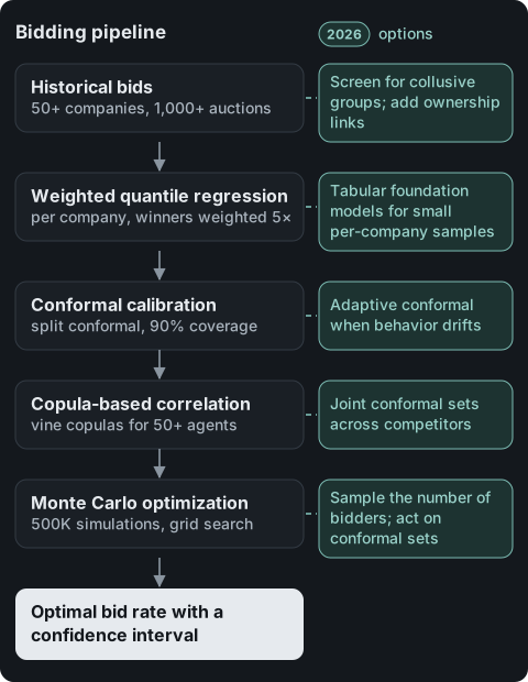
The current pipeline for competitive bidding:

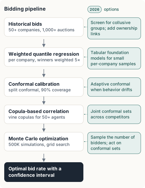
It covers what the matrices ask for:

• it learns behavior from history instead of assuming rationality
• it predicts distributions, not point estimates
• it models correlation between competitors
• it handles one-shot, simultaneous decisions
• it gives guaranteed coverage instead of approximate bootstrap intervals

What changed in 2026

I added this section in October 2026. The matrices above still hold; these developments change how you would apply them. The figures mark them in teal.

Generative auto-bidding went into production

In online advertising, auto-bidding moved from RL toward generative policies trained on logs. AIGB (Guo et al., KDD 2024) trains a conditional diffusion model on whole bidding trajectories and reports a 2.81% increase in GMV and a 3.36% increase in ROI in an online A/B test at Alibaba. Kuaishou followed with several variants:

• GAS (Li et al., WWW 2025): post-training search over a generative policy
• GAVE (Gao et al., SIGIR 2025): value-guided exploration for Decision Transformers
• Diffusion completer-aligner (Li et al., KDD 2026): raised advertisers’ conversions by 2.0% on average at similar spend, compared with the Decision Transformer it replaced in production
• BidFlow (Yang et al., KDD 2026): a flow-matching policy, introduced with the PlatformBid benchmark

Meituan’s GRAD (Lei et al., 2025) pre-trains one large generative model for auto-bidding. A mixture-of-experts module proposes bidding actions, and a causal-transformer value estimator keeps them within cost-per-mille and ROI constraints. Deployed in several of Meituan’s marketing scenarios, it raised GMV by 2.18% and ROI by 10.68%.

The newest work puts an LLM above the bidder. In AIGB-R1 (Dou et al., 2026), an LLM planner sets the strategy and a generative executor places the bids, and both are trained with reinforcement learning in a bidding simulator. So far it has been evaluated offline, on a public dataset.

All of these sit in the repeated, data-rich corner of Matrix 1: an ad platform runs millions of auctions a day and logs every one. They do not change the recommendation for one-shot sealed bids with a few thousand records. They do support Matrix 4: when bids are multimodal, expressive generative models such as diffusion and flow matching beat single-point policies.

LLM agents are now competitors to model

Shah et al. (2025, revised 2026) placed five LLMs in seven laboratory auction settings and compared them with human results from published experiments. The models deviate from theory differently from people, often in the opposite direction: humans overbid in second-price auctions, while most models that deviate underbid. Even so, the three large non-reasoning models keep the human ordering of auction formats by difficulty, and all five reproduce the winner’s curse in first-price auctions. The reasoning model bid almost at equilibrium.

In the Cattle Trade benchmark (Müller and Müller, 2026), which mixes auctions, hidden offers, and bargaining over long games, two heuristic code agents outperformed most of the LLMs tested. The traces show recurring overbidding and self-bidding.

Fish, Gonczarowski, and Shorrer (2026) let LLM-based pricing agents compete in oligopoly experiments. The agents reached prices and profits above the competitive level quickly, without being told to coordinate. Small changes in the wording of their prompts changed how far prices rose, and the results carried over to auctions.

For Matrix 2, this splits the behavioral column. A competitor that hands its bids to a reasoning model moves toward rational play. One that uses a non-reasoning model, or human judgment, stays behavioral, with biases that differ from human ones. When competitors start bidding through agents, their bid distributions shift, so refit the per-competitor models instead of assuming they stay stable. For Matrix 3, agents can become correlated without talking to each other, which is one more reason not to assume independence.

Tabular foundation models change the per-competitor step

Per-competitor models are usually short on data: a contractor may have a few dozen bids. Tabular foundation models help here:

• TabPFN-2.5 (Grinsztajn et al., 2025) handles up to 50,000 rows and 2,000 features. Its regressor returns a full predictive distribution, so quantiles come directly from one model.
• TabPFN-3 (Prior Labs, May 2026) fits up to a million rows with 200 features, or 100,000 rows with 2,000 features, in context.
• TabPFN-3.5 (September 2026) uses one checkpoint for classification and regression and improves the predictive distributions for skewed and zero-heavy targets.
• TabICLv2 (Qu et al., ICML 2026) beats a tuned RealTabPFN-2.5 on the TabArena and TALENT benchmarks without tuning, and scales to datasets with millions of rows.

The TabPFN-2.5 and later weights are released under non-commercial licenses, so a production bidding system needs a commercial license from Prior Labs. Check the license of whichever checkpoint you deploy.

When I modeled public-procurement bids in 2026, I compared TabICLv2, TabPFN, TabM, and RealMLP on chronological splits before choosing a model for each region.

The coverage guarantee still comes from calibration, not from the model, so the conformal step stays:

from tabpfn import TabPFNRegressor

model = TabPFNRegressor()
model.fit(X_train, y_train)
lo, hi = model.predict(X_cal, output_type="quantiles", quantiles=[0.05, 0.95])
scores = np.maximum(lo - y_cal, y_cal - hi)
q_hat = np.quantile(scores, np.ceil((len(scores) + 1) * 0.9) / len(scores))

lo_new, hi_new = model.predict(X_new, output_type="quantiles", quantiles=[0.05, 0.95])
interval = (lo_new - q_hat, hi_new + q_hat)

Conformal prediction is moving into the decision

The pipeline above feeds conformal intervals into a simulation. Recent work ties them to the decision directly:

• Kiyani, Pappas, Roth, and Hassani (ICML 2025) give a decision-theoretic case for prediction sets. For risk-averse decision makers, prediction sets are the optimal form of uncertainty to act on, which is a reason to bid against conformal sets rather than point forecasts.
• Conformal risk training (Yeh et al., NeurIPS 2025) optimizes the model end to end through the conformal risk-control step.

For Matrix 4, regression-as-classification handles multimodal outcomes (R2CCP; Guha et al., ICLR 2024). It predicts a distribution over bins, so the conformal set can split into separate ranges when a competitor might bid either low or high. I used this approach for multimodal bid-rate prediction; the details are in my R2CCP bid prediction project.

Competitor behavior drifts

Split conformal assumes that calibration bids and new bids are exchangeable, and in bidding that assumption breaks over time. Zhang et al. (2025) analyzed the Singapore data from the case study above (2017–2021, more than 8,000 bids from more than 900 contractors). They found statistically significant changes in contractors’ bidding trends over periods of 10 to 20 months, at every level of experience. A model calibrated on last year’s bids is calibrated for last year’s market.

Weighted conformal prediction (Barber et al., 2023) down-weights old calibration data. Online methods go further and adjust after every auction. Adaptive conformal inference (Gibbs and Candès, 2021) widens the interval after a miss and narrows it after a hit, which keeps long-run coverage near the target even when the distribution moves:

alpha_t = alpha  # target miscoverage, e.g. 0.10
for x, y in auctions:  # in time order
    lo, hi = predict_interval(x, alpha_t)
    miss = float(not lo <= y <= hi)
    alpha_t += gamma * (alpha - miss)  # a miss lowers alpha_t, so the next interval is wider

Conformal PID control (Angelopoulos, Candès, and Tibshirani, 2023) extends the same idea with integral and scorecasting terms. Jun and Ohn (2026) also revise past predictions when new data arrive, which adapts faster after a shift and gives intervals up to about 30% narrower.

Correlated bidders: joint sets, ownership links, and screens

Three developments sharpen Matrix 3:

• Joint conformal sets. Park, Tibshirani, and Cho (2024) calibrate one prediction set over several correlated targets. They estimate the joint distribution of the nonconformity scores with nonparametric vine copulas, which scales to many targets and gives asymptotically exact coverage. That is the conformal counterpart of the vine-copula step in the pipeline: coverage for the whole field of competitors instead of one at a time.
• Ownership links. Asai and Charoenwong (2026) matched Singapore procurement auctions with the registered shareholders of every bidding firm. Bidders that share owners, or owners’ owners, are more likely to submit identical bids, and identical bids go with higher contract prices. Some correlation between competitors is coordination, and ownership data can help predict it.
• Collusion screens. Graph neural networks trained on tenders from Japan, the United States, Switzerland, Italy, and Brazil detect collusive patterns better than standard networks, and the authors also test them on markets without training data (Gomes et al., 2024). Convolutional networks flag cartel participants from plots of their bids against competitors’ bids (Huber and Imhof, 2023). Run a screen before fitting the copula, so coordinated bids aren’t treated as ordinary market correlation.

The simulation also needs to know how many bidders will show up. Oo et al. (2025) predict the number of bidders on Singapore construction tenders with explainable machine-learning models, so the Monte Carlo step can sample that number instead of fixing it.

The rational benchmark got cheap

I still don’t use equilibrium to predict competitors (see Methods to avoid), but computing it is no longer the obstacle. SODA (Bichler, Fichtl, and Oberlechner, 2025) discretizes types and bids and learns distributional strategies with online optimization. It closely approximates the known Bayes–Nash equilibria across many auction models and finds them in seconds for standard symmetric ones.

That makes an equilibrium bid a cheap reference point. Measure how far each competitor’s bids sit from it, and watch that gap as competitors start bidding through reasoning models, which Shah et al. found bid close to equilibrium.

Offline RL caught up on multimodal actions

Flow Q-learning (Park, Li, and Levine, ICML 2025) pairs a flow-matching behavior policy with a one-step policy trained by Q-learning. This handles multimodal action distributions without iterative sampling when deciding.

Decision Transformer’s place is less settled:

• Bhargava et al. (ICLR 2024) found it ahead of CQL and BC in sparse-reward settings with low-quality data.
• Omori et al. (2025) found that filtered BC matches or beats it in those same sparse-reward settings, at lower cost.

The guidance above stands: for independent one-shot bids, BC plus simulation is enough. For repeated auctions with large logs, try flow-based offline RL first; it is now the stronger baseline.

MEV block building moves into the protocol

Ethereum’s Glamsterdam upgrade makes proposer–builder separation part of the protocol (ePBS, EIP-7732), so builders bid as recognized participants instead of through off-chain relays. It went live on the Sepolia testnet on October 6, 2026; the mainnet date hasn’t been set.

What to use for how much data

Less than a month

Skip sophisticated methods. Use:

• moving averages of competitor bids
• kernel density estimation
• conservative manual rules

One to six months

• per-competitor models with Random Forest or XGBoost
• bootstrap prediction intervals
• independent simulation

Six months or more

The full pipeline:

1. Features: context such as rank, gap, and competition intensity
2. Per-agent models: quantile regression with winners weighted more
3. Correlation: factor models or copulas
4. Simulation: Monte Carlo with correlation-aware sampling
5. Calibration: conformal prediction for guaranteed coverage

Two years or more

Add:

• clustering competitors by behavior (aggressive, balanced, conservative)
• adjustments per contracting institution
• seasonality and trends
• optionally, diffusion models for multimodal scenarios

Methods to avoid for competitive bidding

Full multi-agent RL

It assumes you can learn through interaction. In real bidding you cannot experiment, because every bid costs money. The exception is a simulator where exploration is safe.

Nash equilibrium computation

It assumes rational agents, and real competitors are behavioral. The exception is a highly liquid market dominated by algorithmic traders.

Pure game theory

It assumes common knowledge of rationality, while real competitors have private information and bounded rationality. The exception is a simple two-player game with known payoffs.

Mean-only predictions

A prediction that a competitor will bid 88.5% is useless without knowing whether the error is ±0.5% or ±3%. Use it only for a first look at the data.

References

1. Albrecht, S.V., Christianos, F., Schäfer, L. (2024). “Multi-Agent Reinforcement Learning: Foundations and Modern Approaches.” MIT Press.
2. Kumar, A., et al. (2022). “When Should We Prefer Offline Reinforcement Learning Over Behavioral Cloning?” ICLR.
3. Angelopoulos, A.N., Bates, S. (2022). “A Gentle Introduction to Conformal Prediction and Distribution-Free Uncertainty Quantification.” arXiv.
4. Romano, Y., Patterson, E., Candès, E. (2019). “Conformalized Quantile Regression.” NeurIPS.
5. Barber, R.F., et al. (2023). “Conformal Prediction Beyond Exchangeability.” Annals of Statistics.
6. Rashidinejad, P., et al. (2021). “Bridging Offline Reinforcement Learning and Imitation Learning: A Tale of Pessimism.” NeurIPS.
7. Czado, C. (2019). “Analyzing Dependent Data with Vine Copulas: A Practical Guide.” Springer.
8. Chi, C., et al. (2023). “Diffusion Policy: Visuomotor Policy Learning via Action Diffusion.” RSS, IJRR 2024.
9. Hu, S., et al. (2024). “HarmoDT: Harmony Multi-Task Decision Transformer for Offline Reinforcement Learning.” ICML.
10. Wang, Y., et al. (2024). “Critic-Guided Decision Transformer for Offline Reinforcement Learning.” AAAI.
11. Ze, Y., et al. (2024). “3D Diffusion Policy: Generalizable Visuomotor Policy Learning via Simple 3D Representations.” RSS.
12. Huang, J., He, N., Krause, A. (2024). “Model-Based RL for Mean-Field Games is not Statistically Harder than Single-Agent RL.” ICML.
13. Omori et al. (2025). “Should We Ever Prefer Decision Transformer for Offline Reinforcement Learning?” arXiv:2507.10174.
14. Lotan, R.M., Talgam-Cohen, I., Romano, Y. (2024). “Statistically Truthful Auctions via Acceptance Rule.” arXiv:2405.12016.
15. Vijayan, S., et al. (2025). “Online Bidding under RoS Constraints without Knowing the Value.” WWW.
16. Su, K., et al. (2024). “AuctionNet: A Novel Benchmark for Decision-Making in Large-Scale Games.” NeurIPS Datasets and Benchmarks.
17. Zhao, J., Qiu, G., Guan, Z., Zhao, W., He, X. (2018). “Deep Reinforcement Learning for Sponsored Search Real-time Bidding.” KDD.
18. Raun, C., et al. (2023). “Leveraging Machine Learning for Bidding Strategies in Miner Extractable Value (MEV) Auctions.” IACR ePrint 2023/1281.
19. Flashbots (2024). “BuilderNet: Decentralized Block Building” and “MEV-Boost: Proposer-Builder Separation for Ethereum.” Flashbots Docs.
20. Singapore Government Procurement Dataset (2015–2021). Ministry of Finance Singapore, Kaggle.
21. Zhang, Y., Oo, B.L., Runeson, G., Lim, B.T.H. (2025). “An Empirical Study of Contractors’ Bidding Trends in Recurrent Bidding: A Case of Singapore Public Sector Construction Projects.” Buildings 15(4), 555.
22. Fazekas, M., et al. (2024). “Global Contract-level Public Procurement Dataset.” Data in Brief.
23. EU Public Procurement Data Space (PPDS) (2024). European Commission.

Added in the October 2026 update:

24. Guo, J., et al. (2024). “AIGB: Generative Auto-bidding via Diffusion Modeling.” KDD.
25. Li, Y., et al. (2025). “GAS: Generative Auto-bidding with Post-training Search.” WWW Companion.
26. Gao, J., et al. (2025). “Generative Auto-Bidding with Value-Guided Explorations.” SIGIR.
27. Li, Y., et al. (2026). “Generative Auto-Bidding in Large-Scale Competitive Auctions via Diffusion Completer-Aligner.” KDD.
28. Yang, S., et al. (2026). “PlatformBid: An Auto-Bidding Benchmark from a Unified Advertising Platform’s Perspective.” KDD.
29. Shah, A., Zhu, K., et al. (2025). “LLM Bidders Preserve the Mechanism-Level Orderings of Human Bidders.” arXiv:2507.09083.
30. Müller, R., Müller, C. (2026). “Cattle Trade: A Multi-Agent Benchmark for LLM Bluffing, Bidding, and Bargaining.” arXiv:2605.14537.
31. Grinsztajn, L., et al. (2025). “TabPFN-2.5: Advancing the State of the Art in Tabular Foundation Models.” arXiv:2511.08667.
32. Qu, J., Holzmüller, D., Varoquaux, G., Le Morvan, M. (2026). “TabICLv2: A Better, Faster, Scalable, and Open Tabular Foundation Model.” ICML.
33. Kiyani, S., Pappas, G., Roth, A., Hassani, H. (2025). “Decision Theoretic Foundations for Conformal Prediction: Optimal Uncertainty Quantification for Risk-Averse Agents.” ICML.
34. Yeh, C., Christianson, N., Wierman, A., Yue, Y. (2025). “Conformal Risk Training: End-to-End Optimization of Conformal Risk Control.” NeurIPS.
35. Guha, E., Natarajan, S., Möllenhoff, T., Khan, M.E., Ndiaye, E. (2024). “Conformal Prediction via Regression-as-Classification.” ICLR.
36. Park, S., Li, Q., Levine, S. (2025). “Flow Q-Learning.” ICML.
37. Bhargava, P., et al. (2024). “When Should We Prefer Decision Transformers for Offline Reinforcement Learning?” ICLR.
38. Lei, Y., Zhao, J., Zhao, Y., et al. (2025). “Generative Large-Scale Pre-trained Models for Automated Ad Bidding Optimization.” arXiv:2508.02002.
39. Dou, Y., Wang, H., et al. (2026). “AIGB-R1: Self-Evolving Generative Auto-Bidding via Hierarchical Planner-Executor Optimization.” arXiv:2607.17281.
40. Fish, S., Gonczarowski, Y.A., Shorrer, R.I. (2026). “Algorithmic Collusion by Large Language Models.” arXiv:2404.00806.
41. Prior Labs (2026). “TabPFN-3” and “TabPFN-3.5” release notes. docs.priorlabs.ai.
42. Gibbs, I., Candès, E. (2021). “Adaptive Conformal Inference Under Distribution Shift.” NeurIPS.
43. Angelopoulos, A.N., Candès, E., Tibshirani, R.J. (2023). “Conformal PID Control for Time Series Prediction.” NeurIPS.
44. Jun, J., Ohn, I. (2026). “Online Conformal Inference with Retrospective Adjustment for Faster Adaptation to Distribution Shift.” Pattern Recognition.
45. Park, J.W., Tibshirani, R., Cho, K. (2024). “Semiparametric Conformal Prediction.” arXiv:2411.02114.
46. Asai, K., Charoenwong, B. (2026). “Ownership Networks and Bid Rigging.” Review of Corporate Finance Studies.
47. Gomes, L., Kueck, J., Mattes, M., Spindler, M., Zaytsev, A. (2024). “Collusion Detection with Graph Neural Networks.” arXiv:2410.07091.
48. Huber, M., Imhof, D. (2023). “Flagging Cartel Participants with Deep Learning Based on Convolutional Neural Networks.” International Journal of Industrial Organization 89, 102946.
49. Oo, B.L., Nguyen, A.T., Ahn, Y., Lim, B.T.H. (2025). “Predicting the Number of Bidders in Construction Competitive Bidding Using Explainable Machine Learning Models.” Construction Innovation 25(7).
50. Bichler, M., Fichtl, M., Oberlechner, M. (2025). “Computing Bayes–Nash Equilibrium Strategies in Auction Games via Simultaneous Online Dual Averaging.” Operations Research 73(2), 1102–1127.
51. Harder, N., Miskiw, K.K., Khanra, M., et al. (2025). “ASSUME: An Agent-Based Simulation Framework for Exploring Electricity Market Dynamics with Reinforcement Learning.” SoftwareX 30, 102176.
52. Ethereum Foundation (2026). “Glamsterdam Testnet Announcement.” blog.ethereum.org.

The Singapore procurement data is available on Kaggle and the GeBIZ portal. Analysis code is available on request.